In the first post in this series, we saw a few examples of natural dynamical systems on the planet – in biology and social dynamics. A dynamical system, we recall, is one whose behavior at any point in time is completely determined by: (1) its current state, and (2) a set of rules that determine how the system evolves from its current state.
The study of dynamical systems arose, like a number of important branches of mathematics, out of physics. In this post, we’ll look at a few examples of dynamical systems in the physical world, then see how some of these display a property known as “sensitivity to initial conditions”, or in common parlance, chaos. From here we’ll work to develop a mathematical framework we can use to model many varieties of dynamical systems. The subject of dynamical systems is actively being developed by applied mathematicians, and has proven a powerful framework for understanding biology, chemistry, physics, and other branches of science.
Moving towards chaos
Some of the most illustrative examples of dynamical systems occur in physics, so we’ll have a look at one of these to begin with.
More on Dynamical Systems
According to Newton’s Law of Universal Gravitation, two masses attract to each other, by gravity, with a force that is directly proportional to the product of their masses and indirectly proportional to the square of the distance between their centers of mass.
In mathematical terms, we can represent Newton’s Law of Gravitation as: [math]F=G\cdot\frac{m_1m_2}{r^{2}}[/math]. F represents the force of gravitation between two objects with masses [math]m_1[/math] and [math]m_2[/math], respectively, that are separated at a distance of r.
Check out this explanation of gravitation in further detail:
Also note this gif image (from wikimedia commons) depicting a small planet orbiting a much larger sun, and note that the sun does not stay still – it is effected by gravity arising from the proximity of the planet.

Since the sun is far more massive than the planet, its position varies only slightly. Likewise, since the real-life sun is far more massive than the Earth and the other planets, its movement is negligible in comparison with the gigantic orbits of its planets. This is described by Newton’s third law of motion, which states that when one body exerts a force of F on a second body, the second body exerts a force of -F on the first body. In shorthand, this is stated as, “for every action, there is an equal and opposite reaction”.
The force the sun exerts on the planets means that there is an equal and opposite force exerted by the planets on the sun, but given the sun’s relatively massive size, this equal and opposite force has only a slight effect on its behavior. In the same way, punching a 90-pound teenager might make the teenager fall down, but delivering the same punch to a 300 pound wrestler will barely make him budge.
The two-body problem
The question of how a system of two celestial bodies behaves is known as the “two-body problem”: given the positions, velocities, and masses of two celestial bodies at some particular point in time, how will the two bodies behave in the future?
The two-body problem is relatively straightforward to understand – Kepler gave a description of the behavior with his three laws of planetary motion, the most crucial of which states that planets orbit the sun in an elliptical shape, not a circle, as was previously thought. The other two laws of planetary motion describe numerically how the orbits behave.
The important point is this: in a solar system consisting only of two bodies, a sun and a planet, it is possible to completely describe the future behavior of the solar system, using Newton’s physics. The system has a known solution.
After the celebrated solution of the two-body problem in the time of Newton, around 1690 CE, the search for a solution to the three-body problem, and the general n-body problem (what happens when there are n bodies in a planetary system, where n is an integer greater than 2), began in earnest.
The three-body problem
In fact, mathematicians quickly realized that the three-body problem is much more complicated than the two-body problem. A system consisting of two planets, or a planet and a sun, is relatively easy to understand, but the presence of a third body makes the sort of straightforward algebraic solution – an ellipse or other conic section – obtained for the two-body problem, impossible. Adding a small asteroid to a two-body system makes a very slight change in the initial situation, but over time, the gravitational effects from the small asteroid compound to create profound changes in the overall system.
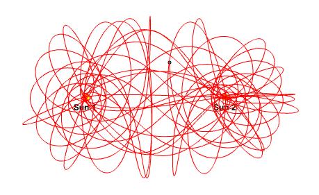
You can play with this collection of 3-body applets to get a feel for the sorts of behavior a 3-body system can display, though keep in mind that these are examples where there’s a clear pattern in the behavior. In general, the behavior of a three body system can be very messy, as the following image of a three body system (with two fixed suns) indicates, made using Newton’s laws at this three-body applet):
In fact, in 1887 the King of Sweden offered a prize to anyone who could solve the general n-body problem, stated as follows:
“Given a system of arbitrarily many mass points that attract each according to Newton’s law, under the assumption that no two points ever collide, try to find a representation of the coordinates of each point as a series in a variable that is some known function of time and for all of whose values the series converges uniformly.”
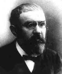
A number of mathematicians feverishly worked on this problem, but it was the prolific French mathematician Poincare (seen in this ClayMath.org image) who finally bagged the prize, ironically by showing why he could not solve it.
Poincare noted that making slight changes in the initial state of a three-body system results in drastic changes in the behavior of the system. This is known as “sensitivity to initial conditions”, and in fact this is the earliest example of a phenomenon exhibiting what is commonly known as chaos.
For 70 years, Poincare’s observation on this characteristic of the three-body problem was obscured, but it came to light again when the mathematician Edward Lorenz noticed that weather systems he modeled on a computer displayed the same property of sensitivity to initial conditions, sparking the field commonly known as chaos theory.
This is commonly visualized as the “butterfly effect”, a term coined by Lorenz, whereby a tiny change in a weather system, such as a butterfly flapping its wings in China – can cause a drastic change in the overall system, such as a tornado in Texas.
What this means for human knowledge
We have seen that it is possible to completely understand the 2-body problem in terms of mathematics; we can develop a system of equations that completely describe the orbit of two celestial bodies. In particular, the orbit of a planet around the sun takes the shape of an ellipse, a conic section that can be thought of as a skewed circle.
For the 3-body problem, however, this is impossible. There is no simple, algebraic way to describe the orbit of any system of three celestial bodies. In practice, this means that the only way to completely understand a system of 3 bodies is to actually watch how their behavior unfolds. We can use a computer to do this, but it’s necessary to actually observe the orbits in order to see what paths they take.
This gif image, from here, depicts one of the “special” cases of the 3 body problem, when there is a clear pattern in the behavior of the system.
In general, however, a 3-body system cannot be described by a closed form set of equations – there do in fact exist slowly converging infinite series solutions to the 3 body problem, but in practice, in order to see how a 3-body system evolves, it’s necessary to simply watch it evolve. In practice, it’s not possible to predict in advance what the system will do, except for special cases such as the one above.
Even though a 3-body system is completely determined by (1) its current state, and (2) rules given by the laws of physics, in practice, we are unable to determine a 3-body system’s behavior in advance. There are certain areas of knowledge that are, in practice, out of the grasp of our knowledge.
For more on what problems like the 3-body problem mean for the limits of human knowledge, check out the work of the Wall Street trader-and-philosopher Nassim Taleb, including the book The Black Swan, which contains a worthwhile discussion on Poincare’s work, as well as the work of others such as Mandelbrot, which we will explore in this and the next post.
Expressing dynamical systems in mathematical form…
In order to get a better understanding of chaotic systems such as the 3-body system, and the “butterfly effect”, we need to develop a mathematical framework useful for modelling dynamical systems. Let’s keep in mind that the definition of a dynamical system is one whose behavior is completely determined, at any given point in time, by (1) its current state, and (2) a rule or set of rules that determine how the system evolves.
In mathematics, such a rule can be given by a function. A function takes an input, perhaps a real number, and applies a rule or set of rules that determines the output of the function. One example is the square function, which takes a real number, multiplies that number by itself, and outputs the result. The square of 2, for example, is 2 times 2, or 4. The square of 3 is 9, and so forth. Mathematically, we represent this rule as [math]f(x)=x^{2}[/math]: f takes any real number x, and outputs its square.
This is just like the sort of rule that determines the evolution of a dynamical system, but in a dynamical system, the rule (or set of rules) is applied repeatedly, over and over again, to determine how the system evolves. The mathematical concept of iterative processes is an ideal framework for modelling such systems.
Iterative processes
An “iterative process” is one in which the same rule is applied repeatedly, using the output as the input for the following iteration. For example, if we take the rule “add 1”, and apply it to 0, we get 1. If we iterate again, we get 2, then 3, and so forth.
Another simple example can be seen with the square function we examined above.
If we take the input 2, then f(2)=4. Applying f again, we see f(f(2))=f(4)=16. Iterating f three times, we see f(f(f(2)))=f(f(4))=f(16)=64. We call the resulting set of numbers the “orbit” of the initial point, 2, under the rule given by f.
If we let f(x)=x^3-1, the function that takes any input, computes its cube, subtracts one, and outputs the result, then, upon iteration of the input 2, we have f(2)=2^3-1=7, so f(f(2))=f(7)=7^3-1=343-1=342, and f(f(f(2)))=f(f(7))=f(342)=342^3-1=40001688-1=40001687.
Got the idea? Iterating a function simply means successively applying the function, using the output as the input for each successive iteration.
You might see a correspondence between iterative functions and dynamical systems. Each of them is determined by a rule that is applied repeatedly to determine the behavior of the corresponding system, or set of numbers, in the case of iterative functions. Iterative functions are therefore a natural mathematical setting for the study of dynamical systems.
Cobweb plot
In many areas of mathematics, there are different ways of representing mathematical concepts; each of which can help us to understand the concept in a different manner.
Given a function f, there is a natural way to map the depict the orbits of a point under the operation of f: a cobweb plot.
Given a graphical depiction of y=f(x), and a starting point [math]x_0[/math], we draw the cobweb plot of the orbit of [math]x_0[/math] as follows:
- Mark the point [math](x_0,0)[/math]
- Draw a vertical line to the point [math](x_0,f(x_0))[/math]. This corresponds to plugging [math]x_0[/math] into the function f.
- Draw a horizontal line to the point [math](f(x_0),f(x_0)[/math] on the line y=x.
- Draw a vertical line to the point [math](f(x_0),f(f(x_0)))[/math]. This corresponds to plugging [math]f(x_0)[/math] into f.
- Repeat the process.
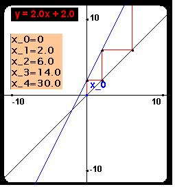
Here’s an example of what happens when we draw the “cobweb plot” for the following functions, starting with the seed value of 0, using the Linear Web applet from Robert Devaney’s website:
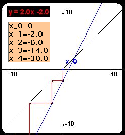
In the above case, as well as the following case, the orbit of the origin “shoots off”, or grows without bound.
Got the idea? Check out this Target Practice game involving the cobweb plot – the goal is to find a starting point whose orbit lands in the given regions. Keep in mind that moving vertically to the graph – say from [math](x, 0)[/math] to [math](x, f(x))[/math] corresponds to plugging the x-value into the function, while moving horizontally, say from [math](x, f(x))[/math] to [math](f(x),f(x))[/math] corresponds to making the previous output the new input.
For the following function, the orbit of the initial point attracts towards a finite point. We call this point a fixed point, since it remains unchanged under the function.
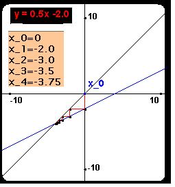
We can solve for the fixed points of a function [math]f[/math] by setting [math]f(x)=x[/math]. In this case [math]f(x)=.5x-2[/math], so the fixed point occurs when x=0.5x-2, ie: when x=-4.
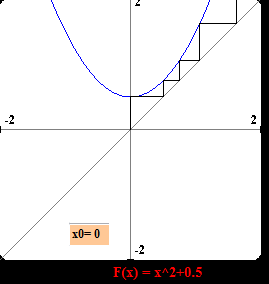
Let’s look at a few examples of cobweb plots for orbits of nonlinear functions, in particular, the family of functions [math]f(x)=x^2+c[/math], where c is any real number.
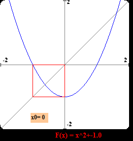
The orbit of the origin under the above function is periodic. [math]f(0)=-1[/math], and [math]f(-1)=0[/math]. It’s periodic with a period of length 2 – after 2 iterations, we are back at the origin.
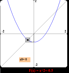
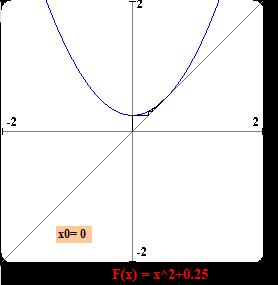
The orbit of the origin under this function above attracts towards the fixed point – we can solve for the fixed point by setting [math]f(x)=x[/math], or in this case, [math]f(x)=x^{2}-0.5=x[/math], yielding the solutions (found by the quadratic equation) [math]x=\frac{1}{2}\pm\frac{\sqrt{3}}{2}[/math]. The fixed point in this case is [math]x=\frac{1}{2}-\frac{\sqrt{3}}{2}[/math]The two fixed points are visible where the graph of the function intersects the diagonal line [math]y=x[/math].
The orbit of the origin under this above function is divergent = it “shoots off” without bound. Like a rocket ship!
And under this function, the orbit of the origin tends towards the fixed point, which turns out to be x=0.5.
Bifurcations
For the quadratic family of functions [math]f(x)=x^2+c[/math], where the real number [math]c[/math] is called the parameter, there are three types of behavior:
- When c<0.25, there are no fixed points.
- When c=0.25, there is one fixed point.
- When c>0.25, there are two fixed points.
In mathematical terms, we say the quadratic family of functions undergoes a bifurcation at c=0.25. Its behavior distinctly changes when the parameter c is varied by a slight amount, around the value c=0.25. Bifurcation literally means “splitting into two parts”, which is what happens with the fixed points of the quadratic family of functions [math]f(x)=x^2+c[/math] at the value c=0.25.
It’s also possible to further categorize these fixed points – in some instances they are “attracting”, meaning the orbits of nearby points tend towards the fixed points, and in other cases they are “repelling”, meaning the orbits of points lead away from the fixed point. This is beyond the scope of this article, but the textbook “A First Course in Chaotic Dynamical Systems”, from Bob Devaney, would be a good starting point.
Chaos
A bifurcation occurs when the behavior of a family of functions undergoes a distinct, qualitative change at a specific value of the parameter. This is very much like what Poincare noticed about the 3-body problem: changing the position, or size, or initial velocity, of any of the planets in a 3-body system, leads to drastic changes in the overall behavior of the system.
Another example of this occurs in the quadratic family of functions [math]f(x)=x^{2}+c[/math], where x and c are complex numbers.
Let’s examine the orbit of 0, the origin, in this family of functions. When c=0, [math]f(x)=x^{2}[/math], so [math]f(0)=0[/math], so 0 is fixed by this function. When c=1, [math]f(x)=x^{2}+1[/math], so [math]f(0)=1[/math], [math]f(f(0))=f(1)=2[/math], [math]f(f(f(0)))=f(2)=5[/math], [math]f(f(f(f(0))))=f(5)=26[/math], and clearly the orbit of 0 grows without bound.
When c=i, then [math]f(x)=x^{2}+i[/math], and [math]f(0)=i[/math], [math]f(f(0))=f(i)=i^{2}+i=i-1[/math], [math]f(f(f(0)))=f(i-1)=(i-1)^2+i=-2i+i=-i[/math], [math]f(f(f(f(0))))=f(-i)=(-i)^2+i=i-1[/math], [math]f(f(f(f(f(0)))))=f(i-1)=-i[/math], and repeatedly iterating f results in a periodic orbit, eventually going back and forth between i-1 and -i.
In general, we can use a computer to check the behavior of the orbit of 0 under any given function [math]f(x)=x^{2}+c[/math]. In fact, the mathematician Benoit Mandelbrot was investigating the properties of this and similar families of functions, just as computers became sufficiently powerful to perform such computations. He plotted the set of values of c in the complex plane for which the orbit of the origin eventually “shoots off” or becomes unbounded (such as c=1), as well as the set of values of c for which the orbit of the origin remains bounded (such as c=0 and c=i).
When he printed out the resulting picture, he was astounded at the image:

When the image is refined, it becomes like this (from here):
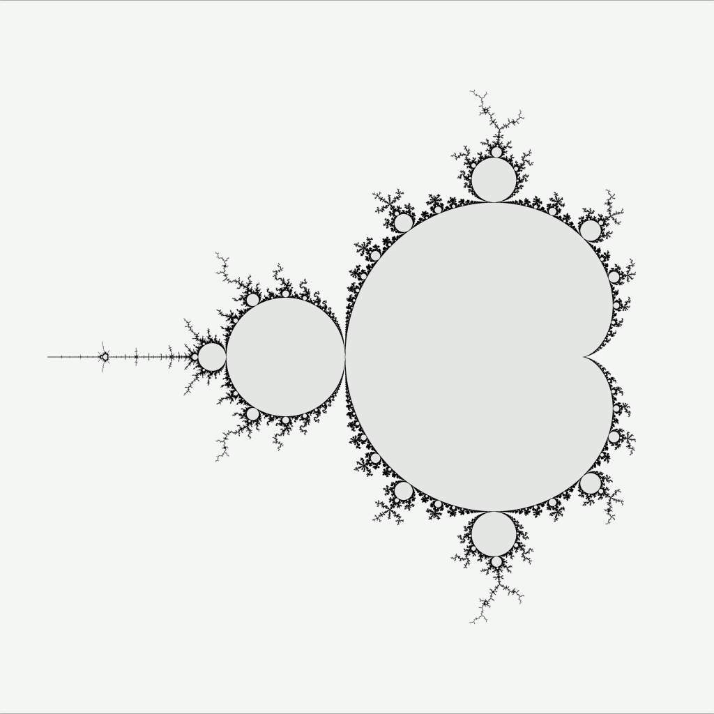
Note that the regions inside the border are those values of c that result in bounded orbits of the origin, while those outside of the border result in “repelling” orbits – for these values of c, the orbit of the origin under [math]f(x)=x^{2}+c[/math] shoots off, like a rocket.
The shape of the border itself is what’s most striking about this set, now well-known as the Mandelbrot Set. A few properties of the set struck le professeur Mandelbrot.
- He noticed that very small changes in the value of c, namely those along the border of the Mandelbrot Set, result in wildly different behavior of the resulting orbits.
- He also noticed that the border of the set isn’t smooth like a circle, but in fact consists of nearly infinite jaggedness – like circles smashed infinitely into each other.
- Finally, he noticed that, zooming in on certain parts of the Mandelbrot Set, yields an image that’s very similar to the original image.
This last property, known as self-similarity, is a key feature of what Mandelbrot termed “fractals” (literally, broken or fractured). You can check out what the Mandelbrot Set looks like in this video of “zooming in on the MS”:
In fact, fractals don’t simply occur in iterative systems such as we have seen – Mandelbrot showed that they in fact describe a wide array of natural phenomena, such as the shape of seashores, river beds, plant growth, and even temporal processes such as fluctuations in the stock markets. They’re not simply abstract mathematical objects, or pieces of artwork, but in fact are key to understanding the structure of the universe.
We’ll see more on this in the third post in this series.
A formal definition of chaos
Mathematics (which comes from the Greek word for ‘knowledge’) has a reputation as being the queen of the sciences, and its ability to uncover truth relies on solid definitions and concrete logic. Definitions provide solid materials on which to build its structure, and logic provides a way to piece together basic concepts into a powerful system of knowledge. Therefore, this post wouldn’t be complete without giving a full and proper definition of chaos. We have only given a loose, informal definition of chaos as a property arising in systems that display sensitivity to initial conditions.
To get a good, usable definition of chaos – one that can be used by scientists to measure the presence of chaos in a system – we need a way to measure sensitivity to initial conditions. If we have a system – a physical system such as an oscillator, or even an abstract mathematical system – we can test its sensitivity to initial conditions as follows:
- Pick a starting point, say [math]x_0[/math]
- Find a point close to [math]x_0[/math], say, [math]x_0 + \Delta x_0[/math]
- Observe how the orbits originating from these two points evolve
This gives an idea about the behavior of orbits originating from nearby points. In order to develop this into a metric, we need to determine what happens to the orbits of points arbitrarily close to the starting point, after arbitrarily long periods of time. If the respective orbits diverge at an exponential rate, then we can say the system exhibits sensitivity to initial conditions.
We can define the Lyapunov exponent, as follows: [math]\lambda = \lim_{t \to \infty} \lim_{\Delta x_0 \to 0} \frac{1}{t} ln(\frac{\Delta x_t)}{\Delta x_0})[/math].
The “ln” or natural log simply measures the rate of exponential growth of the ratio between the distances at time t and time 0, and the entire term, the Lyapunov exponent, gives the average of these. If the Lyapunov exponent is positive, paths beginning arbitrarily close together end up diverging at exponential rates, and thus the system exhibits sensitivity to initial conditions, ie: chaos.
To round the post up…
We’ve introduced one of the central mathematical concepts used to model and study dynamical systems: iterative processes. An iterative process is one in which the same function, or rule, is applied over and over, to each successive result in the process. This is precisely what a dynamical system is – one in which the same rule (or set of rules) governs the change of a system at any given point in time. An iterative process in theoretical mathematics can therefore be used to model a dynamical system in the physical world.
We also have seen how an iterative process can have several types of results – it can result in periodic orbits (one that repeats its behavior), attractive orbits (ones that approach a certain point), or repelling orbits (ones that “shoot off” without bound).
When looking at families of functions, such as the quadratic functions of the form [math]f(x)=x^{2}+c[/math], where x and c are real numbers, the family of functions exhibit a distinct qualitative change at the value c=0.25, resulting in a “bifurcation” at this value of c.
If we examine the complex quadratic functions, those in which x and c are complex numbers, and consider those values of c which result in “tame” (bounded) orbits, we find something similar to the bifurcation idea. Slightly varying the value of c can result in qualitatively different behavior of the orbits. In fact, if we plot out those values of c in the complex plane, we end up with what’s well-known as the Mandelbrot Set. So this relatively simple iterative system in fact exhibits chaos – sensitivity to initial conditions.
This is striking, but provides an illustration of how chaotic behavior seen in real-life systems, such as the behavior of planetary systems, the behavior of double pendulums, and the weather, emerges from relatively simple rules.
We’ll see more about this in the next post, but the striking implication is that the universe is not as smooth and well-behaved as our models have suggested.
As Mandelbrot put it, in his introduction to The Fractal Geometry of Nature, “Clouds are not spheres, mountains are not cones, coastlines are not circles, and bark is not smooth, nor does lightning travel in a straight line.” The study of dynamical systems shows us how this complexity can arise out of deceptively simple foundations.
Leave a Reply to Lê Nguyên Hoang Cancel reply