I’m currently teaching a course on probabilities, which gives me less time to write articles here on Science4All. Yet, it’s made me rediscover the puzzling wonders of probabilities. In particular, in this article, I want to talk about the highly misunderstood concept of conditional probabilities. Starting with this marvel of calculation of conditional probabilities:
“If people cut down the amount of red meat they eat (…) 10 per cent of all deaths could be avoided, they say”. (From this article on EXPRESS.co.uk)
Really think about it… This means that if you cut down the amount of red meat you eat, you have one chance out of 10 to avoid your death! How awesome would that be???
Indeed! I’m actually surprised they still haven’t modified the article! Here’s another more subtle useless statistics: “80 percent of airplane crash survivors had studied the locations of the exit doors upon takeoff. Listen to Neil deGrasse Tyson’s explanation:
More generally, conditional probabilities are often given with one statistics. For instance, it’s sometimes said that a new diagnostic test is efficient at 99%. One might think that this number is impressive. Yet, a single figure is meaningless to describe the efficiency of a test. In fact, later in this article, I’ll present you a 100% diagnostic test that spots all sick people for sure!
The Monty Hall Problem
The most famous confusing problem of conditional probabilities is probably the Monty Hall Problem. At the last round of a game show, you’re faced with three curtains. Behind one of the curtains, there is a car. But the two other curtains hide goats. You’re asked by the presenter to make a first choice. He then reveals one of the curtains you haven’t chosen which contains a goat. The presenter then gives a chance to change your mind and switch curtain. Check Marcus du Sautoy doing the experiment:
So, would you switch curtains?
That’s what the troubling mathematics of conditional probabilities are about! Basically, by removing a curtain with a goat, the presenter has provided new information about the location of the car. This information updates the probabilities for the car being behind each curtain. There are several ways of understanding why the probabilities get changed. Let me first recapitulate du Sautoy’s explanation in the video.
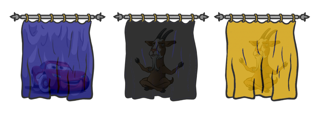
Exactly! Let’s have a figure to redo his reasoning.

Let’s see what happens now if you don’t switch. If you initially chose the blue curtain, you’d win. But if your initial choice is either the black or the yellow curtain, then you’d lose. Overall, by not switching, you win 1 time out of 3.
If you initially chose the blue curtain and you then switched, you’d lose. But now, if your initial choice was the black curtain, the presenter would have to remove the yellow one, and you’d win by switching curtains! For the exact same reason, you’d win too if you initially picked the yellow curtain. Overall, by switching, you win 2 times out of 3.
You’re right. What we’ve been discussing is the chance of winning if you know where the car is and if you pick your initial curtain randomly. Yet, in fact, if you don’t know where the car is, there is still a 1-in-3-chance that the initial pick is right, no matter which curtain is chosen. Thus, the actual case is equivalent to the case where we know where the car is and where we pick the first curtain randomly.
Well, that’s a little bit tricky. Let’s consider the case where we actually don’t know where the car is:

At this point, any choice of the three curtains leads to perfectly similar cases from our perspective. So let’s assume we first pick the blue curtain. Mathematically, we’d say that we can assume having picked the blue curtain without loss of generality. Now, the presenter is going to remove either the black or the yellow curtain. Once again, either case are perfectly similar. So let’s assume that he removes the yellow curtain, once again, still without loss of generality. Thus, we’re left with the blue and black curtains.
Now, to know how probabilities are updated, we first need to track all the cases which may have led to where we are now. Note that the only information we have is that the car is behind the yellow curtain. Thus all the cases could have led to where we are corresponds to those where the car is not behind the yellow curtain. There are two of them:

Without knowing that the yellow curtain has been removed, both cases are equally likely. But, now that we know that the yellow curtain has been removed, and since we know that the first case only leads to the removal of the yellow curtain half of time as opposed to the second case which always does, the second case is twice as likely as the first case. Thus, the first case occurs with probability 1/3, while the second happens 2 times out of 3. Convinced?
OK, let me draw you another picture of what’s going on. Imagine we didn’t know which curtain was removed. Then the following tree displays all the possible configurations.

There are two bifurcations. The first corresponds to the location of the car, the second to the curtain removed. We can compute the probability of each final configuration. Indeed, for a final configuration to occur, the location of the car must match it, which occurs with probability 1/3, and the right curtain must be removed. In the two above cases, this occurs half of the time, while in the two below cases, it’s always the case. The probability of each final configuration is thus obtained by multiplying the probability of the two conditions that lead to it.
Since the yellow curtain has been removed, we know that we must be in one of the two circled configurations. Since the likelihood of the latter configuration is twice as much as the former, it is still twice as likely. This is why the black curtain has twice as much chance to be hiding the car!
Great! The reasoning we have just done here is the seed of the Bayes theorem which we’ll now talk about. But before this, let me provide you a final explanation for the Monty Hall Problem, with this awesome video by AsapSCIENCE:
The great idea of the video is to show you a similar example of the Monty Hall problem where, instead of having three curtains, there are 52 of them. Given your first choice, the presenter removes 50 curtains with goats and suspiciously leaves 1 curtain for you to switch to. Well, instead of curtains, the actually involves cards… Amusingly enough, using greater numbers makes this problem much easier to visualize!
Bayes Theorem
More generally, it often occurs that we try to know a probability of a fundamental fact with the knowledge of its effects. In the Monty Hall problem, the fundamental fact is the location of the car, while its effect is the removal of a certain curtain. Quite often, it’s hard to guess the fundamental fact with the knowledge of its effect. On the opposite, we usually much better understand how the fundamental fact affects the probability of the effect. In the Monty Hall problem, we can describe much better which curtain is going to be removed knowing where the car is.
Yes! Now, because the probabilities of the Monty Hall problem are very simple, they sort of hide the generality of the Bayes’ approach. So let’s consider a new problem of conditional probabilities!
Yes! Let’s do that!
Yes! Very easy. Just tell everyone they are sick! You will have rightly tested all sick patients!
I know! So, just as you’ve pointed it out, the performance of a test clearly requires the knowledge of two figures! I hope that you’ll now rethink twice before judging the quality of a test for which a single number is given! This is precisely the reason why Neil deGrasse Tyson has pointed out that the airplane crash statistics is meaningless.
Yes, let’s get back to this. Consider any test. The way the test is actually rated is based on how it performs on a sample of healthy patients and on a sample of sick patients. What we measure is how often it rightly detects the health of healthy patients, and how it rightly detects the sickness of sick patients. We can draw a similar tree as the one we drew for the Monty Hall problem.

In this figure, the happy man represents a healthy patient, while the man in bed stands for a sick patient. Now, if we take one person at random, the probability of him being healthy is commonly assumed to be the ratio of healthy persons. Given the fundamental fact, what we do understand is how the results will turn out to be. Note that on the figure, a blue thumbs up means that the test says that the patient is healthy. On the opposite, the red thumb down means that the test claims that the patient is sick. Just like before, to obtain the probability of each case at the end of the tree, we need to sum up all probabilities corresponding to arcs leading to the end of the tree. Do you get it?
Now, instead of using words, we are now going to write things down with compact symbols. This will make things easier to manipulate, but the ideas are essentially the same. The major symbol you may not be familiar with is the conditional probability, that is the probability of some event $A$ with the knowledge that an event $B$ has occurred. It is denoted $P(A|B)$. Much shorter to write, right?
Great! Let’s redraw the same figure as above, but with this nice practical notation:

I’m insisting a little bit on this tree, because I think it’s a very nice representation of the complexity of the problem. It works for most problems you need to analyze with conditional probabilities. If you draw this figure, you can avoid a lot of mistakes due to conditional probabilities! Plus, now, we can much easier do reasonings.
Like the probability of a test claiming the patient is sick regardless to whether he is indeed sick or actually not. This corresponds to adding all the end cases which correspond to such a result of the test. Here’s the formula:

This formula, which enables to obtain the total probability of a result given all the possible cases matching the result is called… the law of total probability!
Now, let’s face what’s probably the most important feature of the test: If your test claims that you are sick, what’s the chance of you actually being sick?
Absolutely not! You have inverted what we know and what we want to know! Although data usually describe the conditional probability of the effect knowing the fundamental fact, what we’re often interested in is rather the conditional probability of the fundamental fact knowing the effect. This is the case in our example!
I’m getting there! The probability of a fundamental fact is the ratio of the cases of the fundamental fact which match what we know by all cases which match what we know. This corresponds to Bayes’ theorem:

This formula, which is deduced from all the reasoning we’ve done here, enables us to find the answer to our question with the data we can more easily find. It can be interpreted as the updating of probabilities given new partial information. Somehow, conditional probabilities are often so counter-intuitive and so hard to conceive that it’s practical to just trust the formula and avoid the headache of doing the actual reasoning… But this doesn’t mean you shouldn’t understand where it comes from, and what the operations you’re doing actually mean!
To apply the formula, you need to first compute the probability of a test claiming you are sick. To do so, you need to apply the formula of total probability, which involves the performance of the test both with healthy and sick people. Once again, to judge the performance of a test, you always need to know two figures! Even worse, what we really care about is the probability of the fundamental facts depending on the results of the test. This requires, in addition, to know the probabilities of the fundamental facts with no knowledge of the results of the test. These probabilities simply correspond to the statistics of the fundamental facts which can be obtained by surveys. Find out more with my article on hypothesis tests with statistics.
This understanding of conditional probabilities is essential to the fundamental concept of information. This concept, introduced by mathematician genius Claude Shannon, has revolutionized the world we live in like no other concept ever has. Learn more with my article on Shannon’s information theory.
The Two-Children Problem
Let me finish the article by providing an extremely surprising result, known as the two-children problem or the boy or girl paradox. Note that here, just as quite often, paradox means counter-intuitive, but does not stand for an actual mathematical contradiction!
Consider a man with two kids. One of them is a boy. What’s the probability that the other one is a boy?
At least you did some conditional probability reasoning! To solve this problem, one way consists in applying Bayes’ theorem. But let me provide you the more intuitive approach. There are four possible configurations of the fundamental fact (the sexes of the two kids), which are displayed below, where the taller kid is the older one:

In one of the three cases where one of the children is the boy, the other kid is a boy too. Since all cases are all as likely if no information had been provided, this implies that the conditional probability of the other kid being a boy too, knowing that one is a boy, is 1/3.
Wait there’s more. If the man suddenly says that the boy he was talking about was his older kid, then suddenly the third case of the figure above would no longer be possible. The case where the other kid is a boy suddenly now represents half of the possible case. Thus, just by knowing that the boy he was talking about was the older kid, we would know that the other kid was more likely to be a boy than before!
Wait there’s even more! Let’s get back to another version of the problem: A man has two kids. One of them is a boy born on Tuesday. What would now be the probability that his other kid is a boy?
Hehe… I fell right into the trap when I was given this puzzle by one of my students! I’m now going to provide the answer, so stop reading if you want to search on your own. Of course, we could simply apply Bayes’ theorem, but let me provide a more understandable approach.
When I’m given a problem, I like to draw (even though I’m very bad at it!)… But let’s only draw what’s of interest for us, that is, the cases which correspond to the information we have, namely, a boy being born on tuesday:

And now, to know what’s the probability of the other kid being a boy, we just need to do the ratio of the probability of cases which correspond to the other kid being a boy by the probability of those which still satisfy what we know. This corresponds to dividing the sum of the three first probabilities by the sum of the five. This leads to $(1+6+6)/(1+6+6+7+7)=13/27$.
Indeed, this is! But keep in mind that the only reason this is troubling is due to our poor understanding of conditional probabilities, along with a mistaken common sense.
Sure. What basically occurs is that information about one of the kid sort of subtracts the symmetrical case. Let me explain. The number of cases where one of the kid is a boy is the sum of cases where this kid is the older and of cases where the kid is the younger, minus the symmetrical case where both are boys. Since the other kid can then be a boy or a girl, there are 2+2-1 such cases.
Meanwhile, the number of cases where one of the kid is a boy and the other too is the sum of cases where the former is the older and the cases where the former is the younger, minus the symmetrical case where both are boys. This gives 1+1-1. Thus, the probability of the other being a boy is $(1+1-1)/(2+2-1)=1/3$.
That’s because the numbers are small! Let me do the same reasoning for the case where one of the kid is a boy born on tuesday. Now, the number of cases where one of the kids is a boy born on tuesday is the sum of cases where the kid is the older plus the cases where the kid is the younger, minus the symmetrical case. Since the other kid can be a boy or a girl, born on any day of the week, there are 14+14-1 such cases.
Meanwhile, the number of cases where one of the kid is a boy born on tuesday and the other is a boy too is the sum of cases where the former is the older and the cases where the former is the younger, minus the symmetrical case where both are boys. Because the other kid needs to be a boy, there are 7 possibilities for the latter kid, depending on the day he is born on. This gives 7+7-1=13. Thus, the probability of the other being a boy is $(7+7-1)/(14+14-1)=13/27$.
Somehow, the probability is now closer to 1/2 because the symmetrical case occurs much less often. And it’s precisely the importance of the symmetrical case which makes the conditional probability decrease.
Conclusion
What I hope to have shown you is how bad common sense and intuition are when it comes to dealing with information. It’s not that much about the numbers, but much more about how to deal with what we know and what we don’t know. After all, this is precisely what makes the difference between a good and a bad poker player, as you can read it in my article on Bayesian games, although this setting involves interactions with other players which makes it even more complex. In today’s world ruled by uncertainty, it’s crucial to handle probabilistic reasonings.
I’d like to conclude by a remark on tests. A clever way to make more accurate tests when we’re only able to do not very good ones is to do a sequel of them. This simple idea is key to probabilistic computing and machine learning, as you can find it out in my article on probabilistic algorithms. This has revolutionized technics such as face detection, which basically consists in testing whether a picture contains a face. An accurate of conditional probabilities is essentially for this!
Leave a Reply