Duality analysis holds plenty of additional results in linear programming. In this article, we’ll present the dual variable stabilization, which is a great technic that’s improving linear programming a lot. We’ll consider the smart robber problem I discussed in my article on linear programming. Basically, he has bills and gold to steal, but can only carry a limited volume and a limited weight. Here are the primal and dual spaces in the case of degeneracy defined in my article on duality in linear programming and studied again in my article on simplex methods, when the optimum is stealing bills only.

Dual Variable Stabilization
The concept of dual variable stabilization comes from the context of column generation and the observation that, in cases of high degeneracy, the dual variables had huge oscillation without improvement on the objective function. In our example, in could oscillate between the orange, white and pink dot without improvement. In order to increase speed of algorithms, forcing them not to oscillate was tried. And it worked very well, as it’s shown in the work of Du Merle, Villeneuve, Desrosiers and Hansen (1999), in the work of Oukil, Ben Amor, Desrosiers and Elgueddari (2007), or in the work of Benchimol, Desaulniers and Desrosiers (2011).
As far as I know, what has been missing though is the actual understanding of the reason of the dual variable stabilization success. That is what I’m going to show you here. I’m actually not very aware of the literature on dual variable stabilization, so I have no idea how new my approach is. But I came up with it on my own (well, with help from Hocine Bouarab). Criticisms and questions are more than welcome!
The idea of the dual variable stabilization is to penalize great modifications of the dual variables between iterations of the simplex method. The way it’s done is by allowing small modifications without penalties, and then to add linear penalties for important modification. Just like on the following graph.

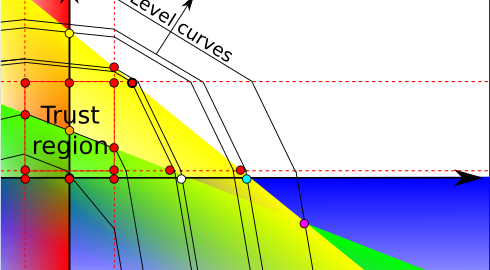
Since the dual program is a minimization program, the program obtained by adding those penalties is a linear program with an objective function that is convex piecewise linear. It can therefore easily be transformed into a linear program that does not have the degeneracy of the initial linear program. Notice that those penalties modify the dual level curves. Suppose we were on the orange dot. This is the graph we’d obtain.

There exists a trust region around the orange dot in which level curves on not modified. This region is defined by upper bounds and lower bounds on variables. These bounds actually define parallel contraints for each variable, drawn by the dotted red lines. Several regions are defined depending on the position regarding the red lines. In each region, the objective function is linear. The intersections of region limits and constraints define new base points. These new base points are drawn in red.
We now use the dual simplex to minimize the linear program that includes penalties. Since, the degenerated space is now much reduced, the dual simplex will quickly get out of the dual space associated with the dual point. As a result, it will quickly reach the dual optimum, which is the bold red dot.
Yes you’re right. In fact, if it’s not in the trust region, we cannot be sure that it’s the optimum of the initial linear program. What we’ll do now is update our trust region and the penalties of the dual space, mainly by centering the trust region around the bold red dot. Here’s what we would obtain in our case.

As you can see, with these new penalties, the bold red dot is no longer the optimum. The bold green dot is. We can obtain it by solving a linear program with these new penalties.
The bold red dot was the intersection of the yellow constraint and the upper dotted red line constraint. With these new penalties, this gives us the bold blue dot. That’s our initial base solution.
By now, you might have realized that primal and dual simplexes are actually two particular cases of a more general simplex that moves from bases to other bases while trying to make both primal and dual solutions feasible.
Precisely! Until we get a linear program with penalties that has an optimum inside the trust region, in which case we’ll know for sure that we’ve reached the optimum of the initial linear program. A next iteration would probably achieve that and show that the cyan dot is the optimum.
As I said, the most important is that the new trust region strictly contains the previous optimum found. But it also seems that the smaller the trust region is, the more quickly we may be able to leave a dual polyhedron with same objective value. But I’m not that sure. Another remark that can be done is that suddenly enlarging trust region is likely to make the last found base solution infeasible, as it’s been done on our example with the bold blue dot. But on the other hand, if the trust region we built was even larger, then the optimum of the initial linear program would have been in the trust region, thus avoiding another iteration.
I’ll also add that choices of penalties are important too. I’m not sure if it has been done, but I’d suggest that the penalties be a vector that is collinear to the vector of costs. This way, if a solution that’s in the top right corner is found, then we’ll know for sure that it’s optimum. Also, there is the matter of whether the penalties should be higher than the initial objective function. If it is, we could totally forbid the bottom left corner, and probably forbid and bottom or left sides. But as a result, there would be less chance to make an interesting move towards the top and right sides, hence increasing the chance of finding a dual constraint base that includes one of the dotted lines, in which case we’ll know for sure that we haven’t reached the optimum.
Well, I guess it’s what needs to be dealt with now. I’m trying to find it, and I’ll add something right here as soon as I can explain it simply… But for that, I first need to understand it myself! Once again, comments and helps are more than welcome!
Let’s sum up
The dual simplex gives a better understanding of the primal simplex. However, both methods face problems of degeneracy. Following this idea though, we could define a more general approach that doesn’t restrict itself to staying in the feasible set (like the primal simplex), nor to keeping reduced costs positive (like the dual simplex). I am actually wondering if there is a way to choose these rules to avoid problems of degeneracy, by allowing a primal pivot towards an infeasible base.
The dual variable stabilization is a great way to deal with degeneracy, as it ensures a quick pivot towards a new feasible point that strictly improves the previous point if the previous point was feasible. Its efficiency has been proved by several experiments on several classical problems.
Leave a Reply