For the last decades, my professors François Soumis, Guy Desaulniers and their colleagues at GERAD in Montreal (where I’m doing my PhD) have made millions of dollars by exploiting two clever mathematical tricks to solve industrial problems. These tricks have become a cornerstone of operations research, the subfield of applied mathematics which involves computational approaches to help decision-making.
The tricks are called column generation and the Dantzig-Wolfe decomposition. They date back from the 1950s. Let’s see how they work.
Sports Team Lineup
Let’s start with an example. Imagine you were the newly appointed president of the GERAD football team. A Qatari foundation has just provided you with seemingly unlimited funds and you are to design the best starting eleven for your football team. In other words, in the huge pool of professional football players, you need to find the best combination of eleven players. And what’s tricky is that these players need to complement one another.
I mean that it’s not good enough to hire the best players. As any football fan knows it, an equilibrium in the team must be met, and complementarities between players must be found. In mathematical words, these nonlinear aspects make the lineup design nontrivial. In more straightforward terms, we need to be smart about how to design the starting eleven. This is where column generation enters in play.
The trouble is that the set of combinations of eleven players is extremely huge. To face this issue, column generation proposes to divide the job of searching for good players (let’s call that recruitment and give it to a recruiter) and the job of selecting among recruited players the best starting eleven (let’s call that the lineup and have a coach doing it). Crucially, because the coach picks up players out of a small set of recruited players, it will be a much easier job for him to find the best starting eleven.
Not only he can. He should. Given the weaknesses of his starting eleven, the coach can direct the recruiter towards the profiles of players that would definitely improve his team. Typically, if a quality defender is missing, the coach should say so, hence signaling the recruiter that he should focus on defenders. Let me recapitulate the column generation procedure with the following figure.
Amazingly, it is. First, because the coach can now really optimize his lineup by testing nearly all possible combinations. The coach’s job is called the master problem. But also and more importantly, his remarks will greatly help the recruiter to pinpoint the promising players who could strictly improve the lineup. The recruiter’s job with the coach’s directives is known as the subproblem. This division of problems into master and sub-problems has enabled great reductions of computation times of optimization algorithms both in exact methods and heuristics. For instance, its applications to integer programming are countless, from logistics to transport, all the way through scheduling and network design.
To go further, I need to tell you about the setting in which column generation was invented and has successfully surpassed all other methods. This context is that of linear programming.
Algebraic Column Generation
Let’s write our linear program as follows:
$$\begin{array}{ll}
\underset{x \in \mathbb R^n}{\text{Minimize}} \quad & c^T x \\
\text{Subject to} \quad & Ax \geq b \\
& x \geq 0
\end{array}$$
We assume that $A$ is a $m \times n$ matrix, which means that our linear program has $n$ variables and $m+n$ inequality constraints. The usefulness of column generation appears when the number of variables is very large. Typically, in vehicle routing, we assign a variable for every possible route. Thus, the number of variables is of the order of the factorial of the number of places to visit.
As illustrated through the sports team lineup problem above, we will define a master problem which will only deal with a small subset of variables. Algebraically, this corresponds to dividing variables into two groups. The first group will be dealt with by the master problem and its elements are called generated columns. Others fall in the second group of non-generated columns.
Algebraically, by reordering variables of $x$ accordingly to the division of variables, we can rewrite the linear program as follows:
Now, computationally, you have to keep in mind that the left complete formulation never appears. The master problem only knows about the right formulation with no non-generated columns. Whenever the subproblem proposes a new variable to add to the formulation, then the main modification to the master problem is the addition of a column to the matrix $A$. This is why column generation is called so.
Through a sensitivity analysis! One powerful aspect of linear programming is the ability to identify the bottlenecks of an optimization, just as our coach has managed to identify the weaknesses of his lineup. This identification can be done pretty straightforwardly using duality. In essence, given the optimal dual variables, the master problem can relate the potential improvement of a non-generated variable $x_j$ by merely looking at the cost $c_j$ of the variable and the column $A_{*j}$ of matrix $A$ corresponding to that variable.
One beautiful aspect of linear programming is that we have different angles to look at it. For one thing, you might wonder what column generation looks like from a dual perspective. Since columns become rows in the dual program, column generation naturally becomes row generation in the dual, which is better known as the cutting plane method that is widely used in integer programming. Plus, if the dual has a Benders decomposition structure with some stochasticity, and we see that the L-shaped method is nothing else than the dual of column generation.
But there’s more than the dual! I now propose to look at geometrical and combinatorial interpretations of column generation.
Geometrical Column Generation
Recall that linear programming corresponds to determining the South pole of a polyhedron, with the Northwards direction given by the vector $c$, as explained below in my talk A Trek through 20th Century Mathematics:
The trouble is that, for high-dimensional polyhedra, the path to the South pole may be a long one.
Algebraically, removing variables from the master problem is actually equivalent to fixing them to zero. In other words, it’s exactly as if we added equality constraints $x_{k+1} = x_{k+2} = … = x_n = 0$ to the initial linear program. Now, geometrically, such equality constraints represents a vector subspace of $\mathbb R^n$. Thus, the master program corresponds to a focus on the intersection of the initial polyhedron with a vector subspace.
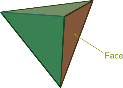
Yes. But not just any sub-polyhedron. Indeed, it’s a vector subspace obtained by saturating some of the inequality constraints defining the polyhedron. Thus, the sub-polyhedron is a $k$-face, that is, a generalization of what 2-dimensional faces of 3-dimensional polyhedra (note that $k$ can be any number between $1$ and $n$). Meanwhile, the Northward direction corresponding to this $k$-face is easily derived as the orthogonal projection of $c$ on the vector subspace.
So, to recapitulate, the master problem of column generation is a restriction of a linear optimization over a polyhedron to the optimization over one of the faces of the polyhedron.
Recall that the master problem focuses on a face defined as the intersection of the initial polyhedron with a vector subspace. Then, the subproblem consists in identifying a direction orthogonal to this vector subspace which may improve the objective value. Crucially, to know whether such a direction $x_j$ is likely to improve the objective value, we need to know additional information about constraints and the Northward direction in this orthogonal direction. These are describes by the cost $c_j$ and the column $A_{*j}$.
Combinatorial Column Generation
Duality teaches us that the concept of base solutions is more fundamental and insightful than that of extreme points. This remark leads me to give you a combinatorial interpretation of column generation.
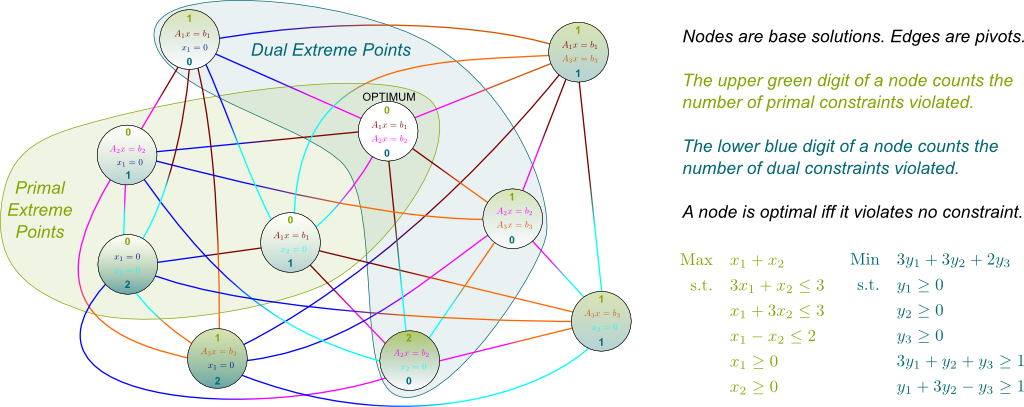
Disregarding rank issues, base solutions are choices of $n$ saturated constraints out of the $m+n$ constraints. Let’s represent each base solution by a node of a graph. Next, let’s link two nodes, if a single pivot is needed to move from the first to the latter base solution. Below is an example where $n=2$ and $m=3$, which also displays the primal and dual feasibilities of base solutions. Note that primal base solutions are exactly primal extreme points.
You may notice that the subgraph made of primal extreme point circles along with edges between these extreme point circles (called the induced subgraph) is a quadrilateral. Indeed, diagonals are not in the graph. This means that the primal polyhedron is a 2-dimensional quadrilateral. Conversely, the dual extreme points are these of an unbounded 3-dimensional polyhedron, which has one triangle face and one edge between its extreme points (as well as several edges pointing towards infinity).
I don’t know how troubling it is, but it is definitely unconventional. Computationally though, it is far from being useful. After all, graphs like the ones above have $\binom{n+m}{n}$ nodes. This is way too many to ever be implemented entirely. However, I do find this representation of linear programming very insightful. For instance, in this representation, the generalized simplex method merely consists of a path along which the numbers of primal and dual violated constraints both never increase. Crucially, while it has no knowledge of the entire graph, the simplex method can enumerate the neighbors of a node to find the best next node to visit. Eventually, it finishes at a node where both numbers are zero, in which case we are at a base solution that is both primal and dual feasible. Such base solution is necessarily primal and dual optimal.
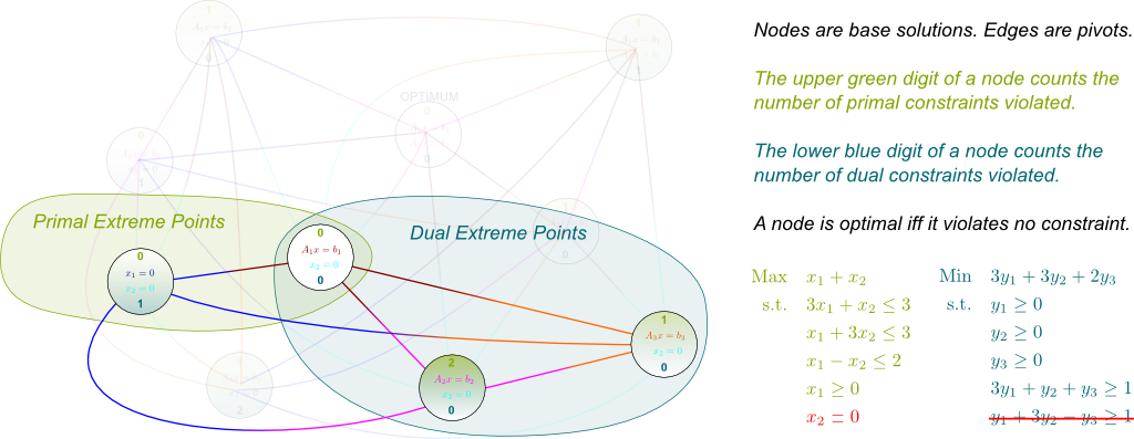
I know! Now, let me finish with what column generation does to this graph. Basically, by forcing non-generated variables to equal zero, column generation focuses on particular induced subgraphs. Crucially, this enables to dramatically reduce the size of the graph we work with. For instance, if we do not generate variable $x_2$ in the example above, we obtain the following induced subgraph:
Notice how column generation affects the dual program: It corresponds to removing a dual constraint. As a result, column generation decreases the number of violated constraints of all nodes. Hence, in the master program, some nodes become dual feasible.
It’s not clear how to illustrate it through our example, as we only had two primal variables here. But the key role of this subproblem is really to find which family of nodes to add such that the optimal node of the master problem is no longer a dual extreme points. In cutting plane method terms, this corresponds to determining a dual constraint which is violated by the dual optimum of the master problem.
Dantzig-Wolfe Decomposition
An article on column generation would not be complete without mentioning the Dantzig-Wolfe decomposition. In fact, from my experience, these two concepts are so often combined that students tend to confuse them. Yet, they are in fact very different ideas. For one thing, column generation is quite universal and applies to all linear programs.
I did. Indeed, column generation always works, but it doesn’t add much unless we have problems with a large number of variables. And by large, I mean exponentially large.
Hehe… There is a clever twist here. In integer linear programming, I’d say that there are 3 main indicators of the difficulty of a problem: The number of variables, the number of constraints and the integrality gap.
The integrality gap is the relative increase in the objective function when we include the integrality condition on variables, as opposed to when we don’t. The greater the integrality gap, the more time it will take to solve an integer linear program.
When the problem has the right structure (and this happens a lot in practice!), it is possible restate the optimization problem to redirect the integrality gap difficulty towards a number-of-variable difficulty, which we can then fight with column generation. This restatement is the so-called Dantzig-Wolfe decomposition.
My professor François Soumis likes to illustrate this Dantzig-Wolfe decomposition with an old project he did. Decades ago, he was asked to infer who voted what from the results of a vote by a board of directors. Given that each director of the board has a known weight in the vote, it is usually possible to do so. For instance, if there are three directors with weights 40%, 35% and 25%, and if the results yield a 65% versus 35%, it is not to hard to guess that the first and third directors voted the inverse of what voted the second one. However, things are not that easy if we now have 15 directors.
We can model the set of possible votes as the integer points of a polyhedron! Let’s call green, blue, orange… etc the alternatives of the vote. Also, we number the directors by numbers 1, 2, 3, … etc. Denoting $w_i$ the weight of director $i$ in the vote, $v_c$ the total of votes for color $c$ and $x_{ci}$ the binary variable which equals 1 if director $i$ votes for color $c$, the fact that all votes for color $c$ add up to $v_c$ corresponds to the constraint $w_1 x_{c1} + w_2 x_{c2} + w_{3} x_{c3} + … = v_c$. Then, for any values of parameters $\alpha_{ci}$, a consistent vote is necessarily an optimal solution of the following integer linear program:
$$\begin{array}
\text{Minimize} \quad & \sum_{c,i} \alpha_{ci} x_{ci} \\
\text{subject to:} \quad & \sum_{i} w_i x_{ci} = v_c \quad & \forall c, \quad & \text{(The votes of directors add up consistently with the observed results)} \\
& \sum_{c} x_{ci} = 1 & \forall i, \quad & \text{(Each director votes exactly once)}\\
& x_{ci} \geq 0 & \forall i,c, \quad & \text{(The last two conditions guarantee that variables are binary)} \\
& x_{ci} \in \mathbb Z & \forall i,c,\\
\end{array}$$
Plus, as you can see, there is a relatively small number of constraints and variables. Indeed, the number of variables for instance is the product of the number of colors by the number of directors. We’re far from the factorial number of routes in vehicle routing problems! Yet…
Yes. And this means that this apparently simple problem can be unbelievably hard to solve.
Exactly! The key idea of the Dantzig-Wolfe decomposition lies in the Minkowski theorem, which says that all bounded polyhedra are convex combinations of their extreme points. In other words, given any polyhedron $P$, denoting $extr(P)$ the set of its extreme points, then points of $P$ can be written $x = \sum \lambda_e e$ with $\sum \lambda_e=1$ and $\lambda_e \geq 0$ for all extreme points $e \in extr(P)$. In particular, $x_{ci} = \sum \lambda_e e_{ci}$. However, this new formulation of the polyhedron $P$ now has as many variables as the number of extreme points of $P$. And that’s a lot. Usually, that’s too many. Even for column generation.
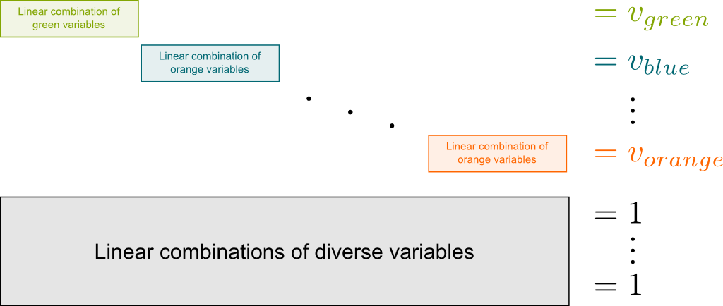
It’s here that it is essential to exploit the structure of the problem. Let’s rewrite the integer linear program by now highlighting where the different variables appear, as we group them accordingly to the colors they correspond to:
The lower black constraints of the representation above are called linking constraints. Let’s forget them for a while. Then, crucially, the matrix $A$ has a striking diagonal structure. Each diagonal block is unrelated to any other diagonal block. The core idea of the Dantzig-Wolfe decomposition is to remark that the whole polyhedron described by all the constraints is the Minkowski sum of the polyhedra that each block describes.
The Minkowski sum $P = \sum P_c$ of polyhedra $P_c$ is the set of vectors $x$ which are sums $x=\sum x_c$ where each $x_c \in P_c$. Importantly, the fact that $P$ is the sum of polyhedra $P_c$ means that it suffices to apply the Minkowski theorem to each polyhedron $P_c$.
Basically, yes.
Now, crucially, we can take the integrality condition into account right here. More precisely, instead of describing extreme points $e^c \in Extr(P_c)$, we are going to list the integral points $e^c$ which are extreme points of $E_c = Conv(P_c \cap \mathbb Z^n)$. This key subtlety is where lies the true power of the Dantzig-Wolfe formulation. Indeed, by considering integrality conditions at this stage, we will greatly reduce the integrality gap, hence making the problem much easier to solve.
That is the question we leave to the subproblem. Actually, given the dual optimum of the master problem, a clever subproblem will even make sure to only generate the promising extreme points. But in our case, it’s actually not too hard to determine all extreme points. Indeed, as it turns out, any decomposition we can do of a vote $v_c$ as an exact sum of some of the weights $w_i$ defines an extreme point $e \in E_c$. This extreme point $e$ is characterized by its coordinates $e_{ci} \in \{ 0, 1\}$ which equal 1 if they include a vote by director $i$ for color $c$. It is also characterized by the color $c$ it corresponds to. We model this latter fact by defining $\delta_{ec} = 1$, by opposition to $\delta_{ed} = 0$ if $d \neq c$.
Using the Minkowski theorem, any point of the polyhedron $Conv(E_c)$ is written $x^c = \sum \lambda_{e^c} e^c$, where the sum is taken over $e^c \in E_c$ and where $\sum \lambda_{e^c} = 1$. All of this can be reformulated as $x^c = \sum \lambda_e \delta_{ec} e$, with $\sum \delta_{ec} \lambda_e =1$, where the sums are now taken for all $e \in E = \bigcup E_c$. But then, we know the total polyhedron $Conv(P \cap \mathbb Z^n)$ is the Minkowski sum $\sum Conv(E_c)$. Therefore, any vector $x$ satisfying all the block constraints is actually $x = \sum x_c = \sum \lambda_e e$, where the weights $\lambda_e$ must satisfy constraints $\sum \delta_{ec} \lambda_e = 1$ for all $c \in C$.
By replacing $x_{ci}$ by $\sum e_{ci} \lambda_e$, we can finally rewrite entirely the integer linear program for variables $x$ as a integer linear program for variables $\lambda$ as follows:
$$\begin{array}
\text{Minimize} \quad & \sum_e \left(\sum_{c,i} \alpha_{ci} e_{ci}\right) \lambda_e \\
\text{subject to:} \quad & \sum_{e} \delta_{ec} \lambda_e = 1 \quad & \forall c, & \text{(Exactly one weight $\lambda_e$ corresponding to color $c$ must equal 1)} \\
& \sum_e \left( \sum_{c} e_{ci} \right) \lambda_e = 1 & \forall i, & \text{(Exactly one weight $\lambda_e$ corresponding to director $i$ must equal 1)} \\
& \lambda_e \in \{ 0, 1\} & \forall e,\\
\end{array}$$
Note that all the coefficients of the constraints are either 0 or 1. In fact, the constraints can be rewritten $B\lambda = {\bf 1}$, where $B$ is a matrix with binary entries and $\bf 1$ is the column vector of 1s. This means that we have a set partitioning problem: Each column (or variable) defines a subset of constraints, and any feasible solution corresponds to a set of columns which partitions the set of constraints.
Crucially, now, the integrality gap can be expected to be much smaller. Indeed, any partition is integral and an extreme points. This hints at the fact that many extreme points are integral. Plus, even though we have a large number of variables, our formulation is now much more manageable by column generation. And, as the story goes, using this Dantzig-Wolfe decomposition, my professor François Soumis managed to give his clients valuable answers to the question of who voted what at a board meeting vote…
They are quite numerous. Most importantly, the combination Dantzig-Wolfe decomposition + column generation has been a powerful approach to solving vehicle routing, shift scheduling and assignment problems.
Let’s Conclude
To recapitulate, column generation relies on a separation of tasks in an optimization algorithm. Namely, it separates the task of proposing interesting alternatives from the task of making the best out of a small subset of alternatives. Amazingly, this simple idea has been monumentally powerful to address industrial problems, and it won my professors millions of dollars. But to reveal the full potential of column generation also requires the use of another clever idea called the Dantzig-Wolfe decomposition. In integer linear programs with great integrality gaps, this decomposition has the great advantage of cutting much of the non-integer points by redescribing polyhedra in terms of convex combinations of (integral) extreme points.
In the last decade, new advancements have come from a clever grouping of constraints. As we enumerate only a tiny fraction of all columns, many constraints become redundant. This means that the problem would remain the same if some of these constraints were simply removed. Because of the very specific set partitioning structure of the Dantzig-Wolfe decomposition, it often turns out that a huge number of constraints are indeed redundant. The dynamic constraint aggregation method is precisely about removing these redundant constraints from the master problem to speed it up.
Exactly. Now, the trouble though, is that, as we generate new columns, we need to figure out which redundant constraints are no longer redundant. At this point, it may be even more clever to redirect the subproblem towards columns which will not require to re-add many no-longer-redundant constraints. This has led to classify non-generated columns into classes of so-called compatibility (which indicates the number of no-longer-redundant constraints one would have to add). The general framework to work this out is called the improved primal simplex (IPS). Finally, one interesting variant of IPS called Integral Simplex Using Decomposition (ISUD) focuses on adding columns in such a way that the optimum of the master problem always remains integral. And all of this is being developed right here in my lab, the GERAD.


Leave a Reply to Lê Nguyên Hoang Cancel reply